Search begins with a deceptively small question: given a query and millions of documents, which documents deserve to appear first?
BM25 remains one of the strongest answers when relevance depends on exact words. It is fast, explainable, requires no labeled training data, and works naturally with an inverted index. Lucene and Elasticsearch use BM25 as their default text similarity; modern retrieval systems frequently keep it beside embeddings because lexical and semantic retrieval fail in different ways.
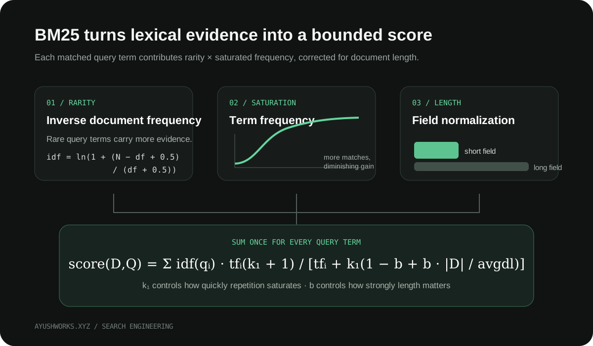
The important idea is not that BM25 “counts words.” It decides how much evidence a word match contributes. A match is stronger when the term is rare across the collection, when it appears repeatedly in the document—but with diminishing returns—and when its frequency is meaningful relative to the document’s length.
The production invariant is:
A relevance score is meaningful only inside the collection, analyzer, field, and query structure that produced it. A BM25 score is not a probability and is not safely comparable across unrelated indexes or queries.
BM25 in one minute
BM25 ranks a document by combining three signals: how rare each query term is across the corpus, how often that term occurs in the document with diminishing returns, and whether that frequency is surprising for a document of that length. The parameters k₁ and b control frequency saturation and length normalization. In production, BM25 is usually executed over an inverted index and evaluated with judged queries—not tuned from intuition alone.
Use BM25 when exact lexical evidence matters: names, identifiers, error codes, product SKUs, API symbols, and specialist terminology. Combine it with dense retrieval when users express the same intent using different words. Fuse independently ranked result lists with a method such as Reciprocal Rank Fusion instead of treating incomparable raw scores as probabilities.
After reading this guide, you should be able to calculate a BM25 score by hand, implement a small ranker, inspect Lucene or Elasticsearch scoring, tune relevance using judgments, and decide when hybrid retrieval earns its operational cost.
The retrieval problem BM25 solves
Let the corpus contain N documents. A query Q contains terms q₁, q₂, …, qₘ. For each candidate document D, the ranker needs a score that increases when the document contains useful query evidence.
A Boolean ranker can determine whether every required term exists, but it cannot express that one matching document is better than another. Raw term frequency helps, but creates a bad incentive: repeating a term 100 times becomes 100 times as valuable as writing it once. Plain TF–IDF recognizes rare terms, yet its frequency and length behavior is often too crude.
BM25 is a bag-of-words lexical ranking function. It does not understand word order, entailment, or semantic equivalence by itself. Its job is narrower: rank documents using corpus statistics and token overlap. That narrowness is a feature. It gives us predictable evidence that an embedding model may miss—identifiers, error codes, names, product SKUs, API symbols, and uncommon technical phrases.
The scoring equation
A common BM25 form is:
                 f(qᵢ,D) · (k₁ + 1)
score(D,Q) = Σ IDF(qᵢ) · ─────────────────────────────────
 qᵢ ∈ Q          f(qᵢ,D) + k₁(1 − b + b·|D|/avgdl)
where:
f(qᵢ,D)is the frequency of query termqᵢin documentD;|D|is the analyzed length of the document field;avgdlis the average analyzed field length in the collection;k₁ ≥ 0controls term-frequency saturation;0 ≤ b ≤ 1controls document-length normalization;IDF(qᵢ)measures how rare the term is across documents.
The formula is a sum because each query term contributes independent evidence. BM25’s probabilistic origins are richer than this operational description; Robertson and Zaragoza’s review connects the practical ranking function to the probabilistic relevance framework and documents the assumptions behind it.
Implementations differ. Lucene computes inverse document frequency as:
                     N − n(qᵢ) + 0.5
IDF(qᵢ) = ln(1 + ───────────────────)
                       n(qᵢ) + 0.5
Here n(qᵢ) is document frequency: the number of documents containing the term at least once. The added 1 keeps the value positive. Other descriptions of BM25 may show a slightly different IDF, an extra query-frequency term, or a constant factor. When reproducing scores, use the exact formula and statistics of the engine you operate.
Part one: IDF measures discriminative evidence
Suppose a corpus has one million documents:
databaseappears in 10,000 documents;theappears in 900,000 documents.
Using Lucene’s IDF:
IDF(database) = ln(1 + (1,000,000 − 10,000 + 0.5) / (10,000 + 0.5))
              ≈ 4.605

IDF(the)      = ln(1 + (1,000,000 − 900,000 + 0.5) / (900,000 + 0.5))
              ≈ 0.105
One match on database carries roughly 44 times the IDF weight of one match on the. This is why analysis matters before ranking. A stop-word filter might remove the; a domain-specific analyzer might preserve C, R, or Go, even though generic tokenization can damage them.
IDF is collection-relative. Add a large body of database documentation and database becomes less rare. Delete documents or move a tenant to another shard and statistics can shift. The score did not change because the document changed; it changed because the evidence landscape changed.
Part two: term frequency saturates
More occurrences should help, but the tenth repetition is not as informative as the second. BM25 encodes diminishing returns through the fraction containing f(qᵢ,D).
Ignore length for a moment by setting b=0. With k₁=1.2, the term-frequency factor is:
TF saturation = f(k₁ + 1) / (f + k₁)| Term frequency (f) | Saturated contribution before IDF |
|---|---|
| 1 | 1.000 |
| 2 | 1.375 |
| 4 | 1.692 |
| 8 | 1.913 |
| 32 | 2.120 |
∞ | k₁ + 1 = 2.2 |
The asymptote is k₁ + 1. Repetition can strengthen evidence, but cannot grow without bound.
k1 determines the shape:
k₁=0ignores term frequency; a present term contributes its IDF;- a lower
k₁saturates earlier; - a higher
k₁lets repeated occurrences matter for longer.
This is a product decision disguised as a numeric parameter. Search over short product titles usually needs repetition less than search over long legal or technical bodies. Do not tune k1 because a blog post recommends a value. Tune it against judgments representing your users’ information needs.
Part three: length normalization asks whether frequency is surprising
Four occurrences in a 60-token support article may be concentrated evidence. Four occurrences in a 4,000-token manual may be incidental. BM25 compares the document length with the collection average:
length normalization = 1 − b + b·(|D| / avgdl)At b=0, length has no effect. At b=1, normalization fully follows the document-to-average length ratio. The common default b=0.75 applies strong, but not complete, normalization.
Length means analyzed token count for the field—not bytes, source characters, visual height, or _source size. Synonyms, stemming, stop-word removal, overlap tokens, and field boundaries therefore change the numbers BM25 sees. Lucene’s default discountOverlaps=true excludes tokens with zero position increment from length, which commonly affects synonym expansion.
Length normalization can punish genuinely comprehensive documents. That is especially visible when a field mixes titles, summaries, comments, and bodies. The better fix is often field modeling rather than changing b: keep semantically distinct text in separate fields and apply deliberate boosts.
Calculate two documents by hand
Consider the query database and these corpus statistics:
N       = 1,000,000 documents
df      = 10,000 documents
avgdl   = 120 analyzed tokens
k1      = 1.2
b       = 0.75
IDF     ≈ 4.605
Document A contains the term four times and has length 180:
K_A      = 1.2 · (1 − 0.75 + 0.75 · 180/120) = 1.65
TFNorm_A = 4 · (1.2 + 1) / (4 + 1.65)
         = 8.8 / 5.65 ≈ 1.558
score_A  ≈ 4.605 · 1.558 = 7.175
Document B contains the term twice and has length 60:
K_B      = 1.2 · (1 − 0.75 + 0.75 · 60/120) = 0.75
TFNorm_B = 2 · 2.2 / (2 + 0.75) = 1.600
score_B  ≈ 4.605 · 1.600 = 7.368
Document B wins despite containing fewer occurrences. Relative to its length, those two matches are stronger evidence. This example also shows why debugging only raw term counts produces wrong conclusions.
A small implementation you can inspect
This TypeScript implementation follows the formula above. It is suitable for learning and tests, not for scanning a production corpus; a real engine uses an inverted index to visit only documents containing query terms.
interface CorpusStats {
  documentCount: number
  averageDocumentLength: number
  documentFrequency: Map<string, number>
}

interface DocumentStats {
  length: number
  termFrequency: Map<string, number>
}

function luceneIdf(documentCount: number, documentFrequency: number) {
  return Math.log(
    1 + (documentCount - documentFrequency + 0.5)
    / (documentFrequency + 0.5),
  )
}

export function bm25(
  queryTerms: string[],
  document: DocumentStats,
  corpus: CorpusStats,
  k1 = 1.2,
  b = 0.75,
) {
  if (k1 < 0 || b < 0 || b > 1)
    throw new RangeError('BM25 requires k1 >= 0 and 0 <= b <= 1')

  const lengthRatio = document.length / corpus.averageDocumentLength
  const normalization = k1 * (1 - b + b * lengthRatio)

  return [...new Set(queryTerms)].reduce((score, term) => {
    const tf = document.termFrequency.get(term) ?? 0
    if (tf === 0)
      return score

    const df = corpus.documentFrequency.get(term) ?? 0
    const idf = luceneIdf(corpus.documentCount, df)
    const saturatedTf = tf * (k1 + 1) / (tf + normalization)
    return score + idf * saturatedTf
  }, 0)
}
The Set is a modeling choice: this version ignores repeated query terms. Some BM25 variants model query-term frequency; query parsers may also generate repeated clauses or boosts. Again, engine behavior is the contract.
The inverted index makes BM25 operationally cheap
Computing every query against every document would be O(N) scoring work. An inverted index changes the access path:
term: database
postings:
  (doc 17, tf 4)
  (doc 92, tf 2)
  (doc 403, tf 1)
For each query term, the engine reads its postings list. The index also stores or derives document frequency, per-document field-length norms, and collection statistics. It merges candidate streams, computes scores, and maintains the top (k) results. Advanced engines use skipping and dynamic pruning to avoid fully evaluating candidates that cannot enter the current top (k).
The architecture matters:
- The analyzer transforms source text into tokens at index time.
- The query analyzer transforms user text into compatible terms.
- The term dictionary locates postings.
- Postings provide document IDs and frequencies.
- norms provide compact field-length information.
- BM25 scores candidates.
- collectors retain the best results.
Most “BM25 problems” are not formula problems. They are analyzer, field, query construction, or corpus problems.
Configure and inspect BM25 in Elasticsearch
Elasticsearch and Lucene default to k₁=1.2 and b=0.75. A custom similarity is configured when the index is created and assigned at field mapping time:
PUT articles-v1
{
  "settings": {
    "index": {
      "similarity": {
        "technical_bm25": {
          "type": "BM25",
          "k1": 1.1,
          "b": 0.6,
          "discount_overlaps": true
        }
      }
    }
  },
  "mappings": {
    "properties": {
      "title": { "type": "text", "similarity": "technical_bm25" },
      "body":  { "type": "text", "similarity": "technical_bm25" }
    }
  }
}
Then inspect a surprising result with _explain:
GET articles-v1/_explain/article-42
{
  "query": {
    "multi_match": {
      "query": "postgresql connection pool",
      "fields": ["title^3", "body"]
    }
  }
}
The explanation tree reveals boosts, IDF, term frequency, field length, and normalization factors. Store these explanations for a small evaluation set during relevance work. They turn “search feels worse” into an inspectable difference.
Changing similarity settings on an existing index requires care because scoring depends on index-time norms and collection statistics. Treat a relevance change like a schema migration: create a versioned index, reindex, replay evaluation queries, compare metrics and critical examples, then move an alias.
Fields are separate evidence channels
A title match and a body match do not mean the same thing. A practical query often combines fields:
{
  "multi_match": {
    "query": "retry budget",
    "type": "best_fields",
    "fields": ["title^4", "summary^2", "body", "tags^3"],
    "tie_breaker": 0.2
  }
}
Field boosts are part of the ranking model. They should reflect product semantics, not compensate blindly for bad results. If tags are editorially controlled, a tag match may be reliable. If users can stuff tags, a large boost creates an abuse channel.
BM25F is a formal multi-field extension. Lucene also exposes combined-field behavior for scoring term statistics across fields. Whichever mechanism you choose, document the unit of evidence: a match in title, body, author, and tenant_private_notes must not be treated interchangeably.
Shards can change the statistics
Distributed search introduces a subtlety. IDF and average field length require collection statistics. If each shard computes them from its local subset, scores can vary with shard composition, especially for small or skewed indexes.
Elasticsearch can use a distributed frequency phase (dfs_query_then_fetch) to gather more global statistics before scoring, at additional latency and coordination cost. This is not automatically the right default. Large, evenly distributed corpora usually have similar shard statistics; tenant-per-shard or small collections may not.
The operational test is simple: move the same documents across different shard layouts and compare the top results for critical queries. If rankings move materially, either gather global statistics, improve routing, reduce shard skew, or accept the behavior explicitly.
Tuning BM25 without fooling yourself
Do not optimize k1 and b against a handful of favorite queries. Build a judgment set:
- sample real information needs, not merely raw query strings;
- include navigational, exact-identifier, broad topical, and long-tail queries;
- label graded relevance where possible;
- split tuning and evaluation queries;
- preserve critical “must win” and “must not appear” cases;
- record analyzer, mapping, corpus snapshot, and engine version.
Measure ranking, not clicks alone. Common offline metrics include:
- Precision@k: how many of the first (k) results are relevant;
- Recall@k: how much known relevant material appears in the first (k);
- MRR: how early the first relevant result appears;
- nDCG@k: rewards placing highly relevant documents near the top;
- MAP: averages precision at relevant positions across queries.
TREC’s Deep Learning track uses judged collections and metrics such as nDCG to compare lexical and learned ranking systems. Pyserini publishes reproducible BM25 workflows over standard corpora, which is useful for learning what a defensible experiment looks like.
Online evaluation adds behavior but also bias. Position affects clicks. Zero-result queries may disappear from click-based datasets. A ranking that increases clicks may still reduce task completion. Use interleaving or controlled experiments, and pair behavioral metrics with guardrails such as reformulation rate, abandonment, latency, and downstream success.
Common mistakes
Treating the score as confidence
A score of 12 is not “twice as relevant” as 6 and does not mean 12% or 12 units of confidence. It is an ordering signal generated by one query against one index state.
Ignoring the analyzer
BM25 scores tokens, not source strings. Lowercasing, stemming, synonyms, n-grams, decompounding, and stop words determine which evidence exists. Always inspect analyzed tokens for failed queries.
Mixing fields with radically different length distributions
Concatenating title, body, comments, and metadata creates a length signal with unclear meaning. Separate fields preserve interpretable evidence and tunable boosts.
Tuning parameters before fixing retrieval
If the relevant document is absent from the candidate set because the analyzer removed an identifier or the wrong field was queried, no k1 value will recover it.
Comparing scores across queries
Different terms have different IDF values and candidate populations. Use rank positions or query-normalized features when combining downstream signals.
Forgetting access control
Filtering unauthorized documents after top-(k) retrieval can return too few results and leak distributional information. Apply tenant and authorization filters inside candidate retrieval.
BM25 and dense retrieval are complements
Dense embeddings can retrieve semantic matches with little token overlap. BM25 can retrieve precise lexical evidence without model inference. A strong production design frequently uses both:
query
  ├── analyzer ──► BM25 top 200
  └── encoder  ──► vector top 200
                       │
        reciprocal-rank fusion
                       │
             reranker top 50
                       │
                 return top 10
Reciprocal rank fusion avoids comparing incompatible raw score scales:
RRF(d) = Σ 1 / (k + rankᵣ(d))
         r ∈ retrievers
For retrieval-augmented generation, BM25 is especially useful for exact symbols, policy clauses, versions, and error messages. Dense retrieval helps when the user describes a concept using different words. The reranker can then spend expensive computation on a bounded candidate set.
Hybrid retrieval is not automatically better. It adds index cost, latency, failure modes, fusion parameters, and evaluation work. Start with the failure classes visible in your query set. Add a second retriever when it repairs a measured weakness.
Production review checklist
Before shipping BM25-backed search, answer these questions:
- What unit is ranked: document, passage, product, comment, or field?
- Which analyzer produces index and query terms?
- Which terms, identifiers, and languages must survive analysis?
- What are the field-length distributions and sources of skew?
- Are
k1,b, boosts, and tie-breaking policies versioned? - Can an operator explain a result using term and field evidence?
- Are tenant and authorization constraints applied before ranking?
- Does the judgment set represent real user tasks and long-tail failures?
- How do shard statistics affect small or skewed collections?
- What is the rollback path for an analyzer or relevance change?
- Which exact-match failures justify lexical retrieval beside vectors?
- Which latency and cost budget constrains candidate count and reranking?
The CTO-level conclusion
BM25 is valuable because it turns three defensible intuitions into a cheap ranking function:
- rare terms carry more information;
- repetition helps with diminishing returns;
- frequency must be interpreted relative to document length.
But the formula is only one layer of the system. Relevance is produced by corpus boundaries, analyzers, field modeling, query construction, shard statistics, access filters, candidate generation, and evaluation discipline. A team that changes k1 without understanding those layers is tuning a symptom.
Start by making lexical evidence observable. Inspect tokens. Calculate a score by hand. Build a small judgment set. Version every relevance change. Then decide whether BM25 alone is sufficient, whether field-aware ranking is needed, or whether semantic retrieval repairs a real failure class.
That is the durable lesson: ranking quality does not come from a fashionable model name. It comes from making evidence, constraints, and evaluation explicit.
References
- Stephen Robertson and Hugo Zaragoza, The Probabilistic Relevance Framework: BM25 and Beyond.
- Apache Lucene,
BM25SimilarityAPI. - Elastic, Similarity settings and BM25 parameters.
- Pyserini, reconstructing and scoring BM25 vectors.
- NIST TREC, Deep Learning Track overview.
Related on this site: filtered vector search is a recall budget, RAG quality starts with retrieval evidence, and cache invalidation is a consistency protocol.